|
|
Welcome to the EpiChIP websiteDaniel Hebenstreit1, Muxin Gu1, Syed Haider2, Daniel Turner3, Pietro Lio2, Sarah Teichmann1 1 Laboratory of Molecular Biology, Medical Research Council, 2 Computer Laboratory, University of Cambridge, 3 Wellcome Trust Sanger Institute |
This is a step-by-step quick start tutorial of the ChIP-Seq analysing software EpiChIP.
Before you start may want to make sure:
- You have downloaded EpiChIP. If not you can download it
here.
- You have been through the introduction and know what EpiChIP does in general.
here.
- You have Java 1.6 (Java 6) or higher on your platform. You can check out your Java version by executing this line in command shell:
java -version
Once you have met all requirements go head.
There is no need of any input files to go through this - the demo files (Chromosome 1 of mouse Th2 H3K9/14ac and IgG control data) include all. And note that this tutorial only takes you through all the features of our EpiChIP - it does not explain very much what EpiChIP does in detail. In order to find out the technical details you may refer to the documentation.
Step 0: Start up
Run the file EpiChIP_Version.jar by typing the command line "java -jar -Xms256m -Xmx512m EpiChIP_Version.jar" under the EpiChIP directory (replace "EpiChIP_Version.jar" by the file name of the JAR file under EpiChIP directory).
Once launched the programme, you should see an interface like this:
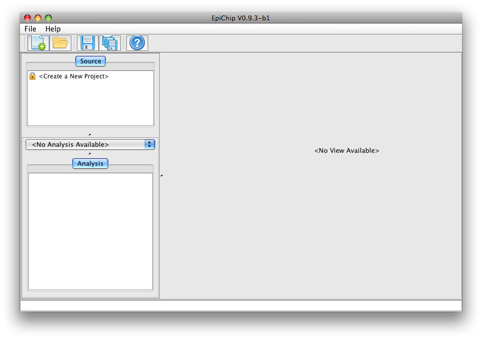
Step 1: Create a new Project
Click on the "File" menu. Select "New Project" item.
You should see a pop-up box asking for a project name. Enter a name here and click "OK".

Step 2: Import experimental data
Now you should see a tree in the top left area of the main window. Click the "<Import Experimental Data>" item in the tree. In the next step, you will need to supply EpiChIP with two files: 1) ChIP-seq reads 2) Gene Annotation.

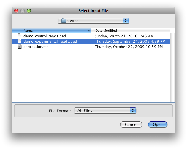
On clicking, a new window will pop up asking for input file and gene annotation.
Click the "Browse" button in the upper half and select "demo_experiment_reads.bed" in the default "demo" folder.
Make sure the gene annotation box in the lower half is on "mouse_mm9_refseq".
Then click "Next" button.
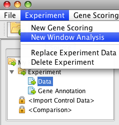
Step 3: Add a window analysis - (Searching for windows amongst genes, exons and introns)
Click on the "Experiment" menu, then "New Window Analysis" item. These analyses will generate the overall read landscapes along genomic objects (genes, exons, introns).
Then click the "Run" button.
(Warning: for each box you check, it will take up to 10 seconds.)

Step 3-1: View and rank the windows
In the bottom left tree, click on the "View All Windows" item. Subsequently, the windows will be identified from the read landscapes.
Each row in the table is a window, and the table is ranked by % bases within the window (5th column).

Step 4: Gene scoring analysis - (Get histone modification for each gene)
Now you should have some ideas about the optimal window and you want to use it to get the epigenetic modification level for each gene. click the "Experiment" menu and then click "New Gene Scoring" item. In this analysis, a score will be calculated for each gene on the specific window, indicating the extent of histone modification level.

The pop-up window ask for the window of each gene to score the reads against. The default setting is the 1kb window from 5' ends of genes. For now, do not change any parameters and click "Run" (If you have run the "Window Analysis" and know where the optimal window is, you can adjust the parameters to the optimal window)

Once finished, click on "Result - Density Plot" to view the distribution of NLCS values. Adjust "Bandwidth" above the graph to alter the smoothness of the distribution (this does not affect the analysis). You will probably noticed the distribution consists of two distinguishable peaks.

Step 4-1: Curve Fitting - (Separate the noise from background)
The distribution of epigenetic scores for all genes usually consists of a mixture of noise and signal. This sub-analysis is dedicated to parameterise the two individual distributions and to separate them.
In the tree that is in the bottom left area of the main window, click on the "<Fit Curves>" item.


Once the curve model has been established, you may see which genes are classified as signal or noise by clicking "View Clusters". You may choose the curve types and desired FDR from the boxes on top of the table.

Step 4-2: Correlation (Link epigenetic modification data to gene expression data)
Click on "<Find Correlation>" item in the same tree. A box will pop up. Select the file "expression.txt".
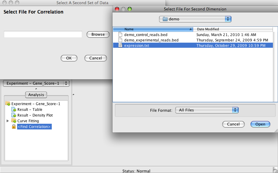
By now you should be able to see a 2D x-y scatter plot and a 2D heat map.
Step 4-2-1: Select a group of genes
In the bottom left tree, under "Correlation" tree node, click the item "<Select Groups>".
In the pop up window, draw as many polygon as you like in the left hand side graph. Use left mouse click to draw and right click to finalise. Then EpiChIP will extract the genes that lies in each polygon.
Once done click "Finish" button.

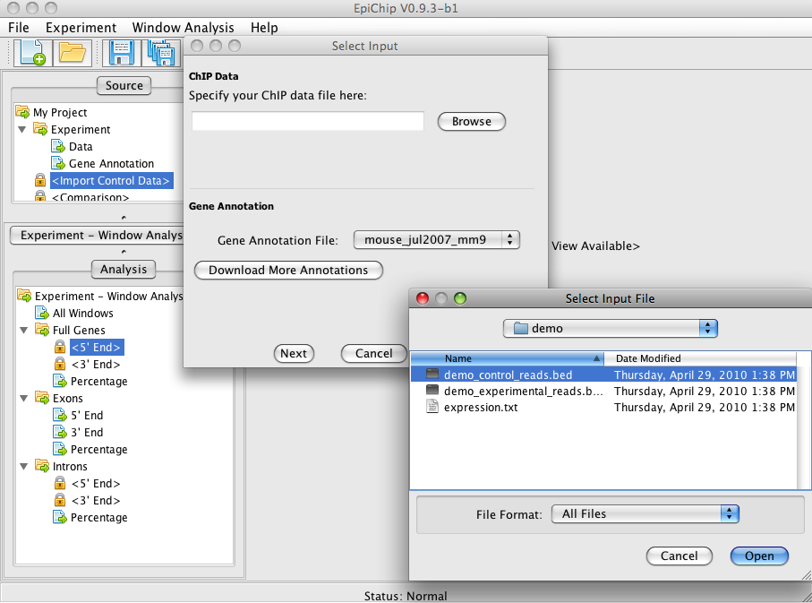
Step 5: Import Control Data
In the top left tree, click on "<Import Control Data>" item. Select the file "demo_control_reads.bed".
Step 5-1: Window analysis of control
In the "Control" menu, click on "New Window Analysis". Untick some boxes and click "Run" button. (Same as before.)
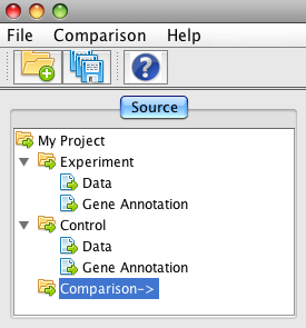
Step 6: Compare experiment with control
Make sure you HAVE done all the steps above, especially you HAVE created a Gene Scoring analysis in the Experiment and a Window Analysis in BOTH Experiment and Control. If you have, in the top left tree click on the item "Comparison" - it takes few seconds to run.
You can see the comparison for gene scoring by selecting "Comparison Gene_Score-#" in the drop-down box.
OR you can see the window analyses comparison by selecting "Window Analysis" from the drop down box.

Saving the Results
Whenever there is a table or graph, you can always save it by clicking the You may also save the whole project by clicking "File (Menu) -> Save Project" and open in the future.
Summary
Thanks for reading this guide and I hope it helps you get off a good start in using this software. Feel free to explore the details of these features and I'm sure there are a lot more you can find out.
Finally, I wish thee good luck and hope you enjoy using EpiChIP as much as I have enjoyed creating it. I look forward to seeing it be of help to your publication.