Contents

0 Installing EpiChIP
1 Creating a New Project
        1.1 Input File Format
        1.2 Gene Annotation File
2 Method Description
        2.1 Window Analysis
                2.1.1 Read Landscape along Genomic Object
                2.1.2 Identification of Windows
        2.2 Gene Scoring Analysis
                2.2.1 Curve Fitting
                2.2.2 Integration of a Secondary Data Set
3 Software Infra-structure
        3.1 Project
        3.2 Experiments
        3.3 Major Analyses
        3.4 Sub-analyses
4 Troubleshoot

Glossary

Bases - For example, 10 extended reads (to 200 bp) correspond to 2000 bases
Curve Fitting - A Sub-analysis that belongs to Gene Scoring. It separates the bimodal distribution
Gene Scoring - A Major Analysis that calculats the NLCS for each gene
Genomic Object - Either a gene, an exon or an intron in the context of Window Analysis
Genomic Mark - The 5' or 3' end of a genomic object
NLCS - Normalised Locus-specific Chromatin State, an indication of the level of hisone modification for a window (NLCS - read bases/ total read bases * 10^6)
Window - A region within a Genomic Region where read enrichment is especially high. (i.e. where epigenetic modification occurs)
Window Analysis - A Major Analyses where the windows of Chip-seq reads are identified

0. Installing EpiChIP

Download EpiChIP from download page. Then unzip it. Make sure you have java 1.6 or above on your computer (if you have problems, please refer to the FAQs).

1. Creating a New Project

First of all, launch the EpiChIP GUI by typing "java -jar -Xms256m -Xmx512m EpiChIP_Version.jar" under the directory of EpiChIP (replace "EpiChIP_Version.jar" by the file name of the JAR file under EpiChIP directory).

Once the EpiChIP GUI has been successfully lauched and a project has been created, either the Experiment or Control (or both) needs to be created in order to proceed. Creating an Experiment or Control requires two input files: the ChIP-seq data file which is provided by the user and the Gene Annotation file which can either be downloaded from the software or generated by the user themselves. Both ChIP-seq data file and Gene Annotation file have to meet certain requirements.

1.1 Input File Format

BED file of UCSC Genome Browser and the output of mapping software Maq, Bowtie and Eland are guaranteed to work for EpiChIP. In a general case, EpiChIP accepts input files as long as they meet the following standards.

If the input file is in BED format (UCSC Genome Brower), it is always accepted and interpreted as:
- each line is a sequencing read
- the first column is the chromosome
- the second column is the lower boundary (inclusive) of the read
- the third column is the higher boundary (inclusive) of the read

If the input file is the output of a mapping software, it will be accepted if and only if:
- each line represents a sequencing read
- it contains only 1 column of chromosome ("Chr#" case insensitive, where # stands for chromosome number)
- it contains only 1 column of strand ("+/-" or "F/R")
- it contains only 1 column of the starting position of the read

1.2 Gene Annotation File

1.2 Gene Annotation File
The Gene Annotation files are preprocessed files containing the genomic coordinates of genes, exons and introns. In order to generate custom Gene Annoation files, one needs to provide the AutoGen.jar module with a file satisfying following conditions (Typing "java -jar AutoGen.jar" also displays the following text.).

- Line 1: Header
- Line 2 onwards:
    - Column 1: Gene Name
    - Column 2: Chromosome
    - Column 3: Strand (+/-)
    - Column 4: Gene Lower End (inclusive)
    - Column 5: Gene Higher End (inclusive)
    - Column 6: Coding Region Lower End
    - Column 7: Coding Region Higher End
    - Column 8: Exon Count
    - Column 9: Exon Lower Ends (comma separated)
    - Column 10: Exon Higher Ends (comma separated)
    - Column 11: Alternative Name
    - Separation: TAB
Example:
"NM_001011874 chr1 - 3204562 3661579 3206102 3661429 3 3204562,3411782,3660632, 3207049,3411982,3661579, Xkr4"

Run the AutoGen module in the EpiChIP directory with the annotation file as argument (type "java -jar AutoGen.jar <Annotation_file>" in the EpiChIP folder). The new annotations will then become available in EpiChIP when loading in the input data file.

2. Method Description

2.1 Window Analysis

The first Major Analysis is known as "Window Analysis" where the programme looks for commonalities of ChIP-Seq enrichment in important genomic regions such as the 5' or 3' ends of gene bodies, coding region, exons and introns. It firstly generates a ChIP-read landscape along the given genomic object and then the windows are identified by peaks on each ChIP-read landscape as described in following paragraphs.

2.1.1 Read Landscape along Genomic Object

First of all, the read landscapes (position vs read bases) are calculated for each genomic object from the ChIP-seq data. Then all the genomic objects are aligned according to either their 5' or 3' ends and then their read landscapes are averaged on each base pair relative to the alignment point. These are designated as "5' Lineup" and "3' Lineup" in the software. Additionally, the genomic objects are stretched and compressed to the same length and their modified landscapes are subsequently averaged so that another set of landscapes are generated. These are known as the "percentage Lineups" in the software.

2.1.2 Identification of Windows

Upon these landscapes, windows, if in present, are detected by any region with read enrichment of higher than 40% of the highest point and no less than 150bp in width (2% in the case of percentage length). Once the windows are identified amongst all the genomic marks, their importance is determined and ranked by how many bases fall into each window normalised to the window width.


Sample Analysis (mouse Th2 H3K9ac):

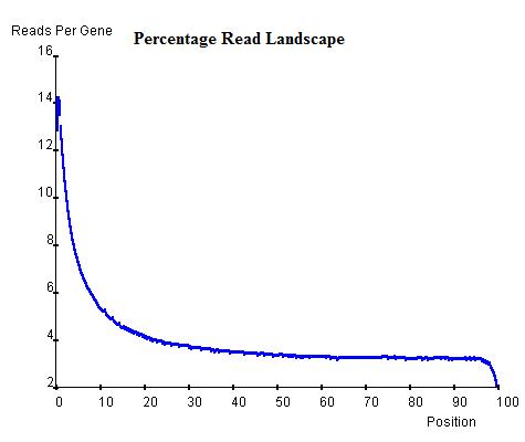
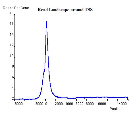
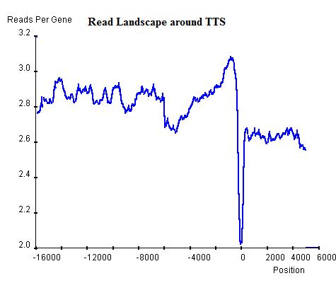
Once the read landscape along genes (exons or introns) has been depicted, histone modification sites are distinguishable from genomic background by showing a strong peak of sequencing reads. In the Th2 H3K9ac data we provide, the landscape around TSS of genes (top-left) indicates a background level of approximately 3 read-nucleotide per gene per base position whereas the peak around TSS shows up to 16 read-nucleotide per gene per base position on average, which suggests a commonality of histone modification sites around TSS that is contributed by a considerable number of genes. On the other hand, the landscape around Transcription Stop Sites (top-right) shows no distinguishable peak but confirms the background level (2.8 read-nucleotides per gene per base position) and the landscape by percentage(bottom) also confirms both the TSS peak's existence and the background read level.

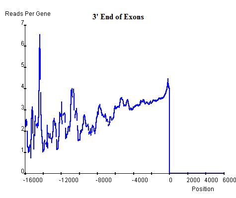
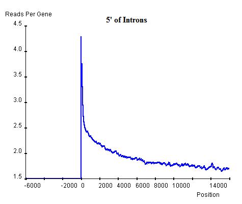
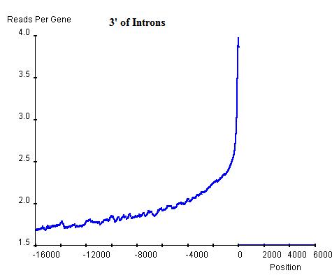
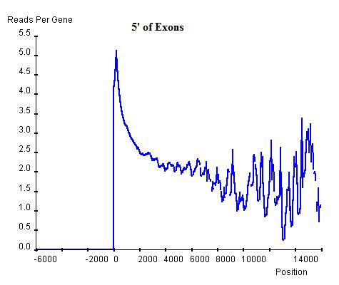
Similarly, the commonality in modification sites (windows) can be investigated at exon-intron and intron-exon boundaries. In exon-intron boundaries (3' end of exons and 5' end of introns, top-left and top-right respectively) it can be seen that towards the end of exons the read enrichment rises from the exonic background, approximately 3 read-nucleotides per exon per base position, to 4 read-nucleotides per exon per base position and once it exits the exon and enters the intron, the enrichment starts to drop sharply until it reaches the intronic background level, approximately 2 read-nucleotides per intron per base position. Similar windows can be found at intron-exon boundaries (3' end of introns and 5' end of exons, bottom-left and bottom-right respectively), indicating the existence of windows at exon-intron and intron-exon boundaries. However, these windows are relatively lower than the window around the TSS of genes and hence can be regarded as secondary windows.

2.2 Gene Scoring Analysis

Gene Scoring analysis is where the NLCS value for each gene is calculated from the specific window. When the window is on the gene body, NLCS for a gene is calculated by the bases of ChIP-seq reads that fall into this window normalised to every million reads and then normalised to every thousand bases of window length. When the window is on either exons or introns, the NLCS for a gene is further normalised to the number of exons or introns within this gene.

2.2.1 Curve Fitting

In the case that the distribution of NLCS values shows bimodality, Curve Fitting provides a mathematical model to parameterise and separate the two subpopulations.

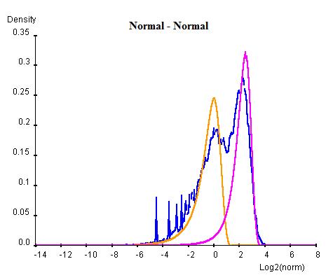
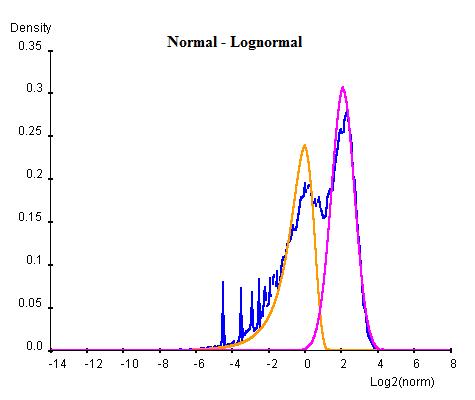
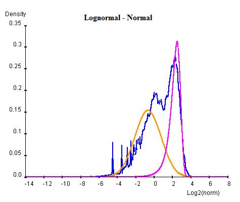
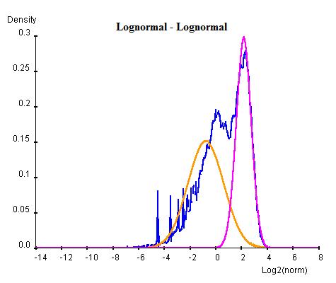
Curve Fitting consists of an Estimation Maximization (EM) method of iterations of Maximum Likelihood Estimations (MLE). In this method each combination of normal or log-normal is executed at one time. For each combination, the whole population of NLCS values are first arbitrarily divided into two groups and two curves of the desired types are parameterised for each group by MLE. Once the two curves have been obtained, the population are re-classified into two new groups by considering which curve has higher probablity of containing each gene. This procedure is repeated for a number of cycles until the sizes of two population become steady. For each cycle, Bayesian Information Criterion (BIC) is calculated as an indication of goodness of fit and the cycle with the lowest BIC is selected as the final result (lower BIC suggests the curve fits better to the data).

Once the BG (background) and HM (histone modification) distributions have been parameterised, a minimum threshold of NLCS above which genes may be classified as HM can be calculated within a desired False Discovery Rate (FDR) by considering the probability of finding a BG above the threshold. Similarly, the BG genes within a given FDR can be obtained by a maximum threshold. Genes having significant probability (FDR less than desired FDR) to be either signal or noise are marked as "overlap" whereas the genes that are significant enough to be neither signal or noise are marked as "unclassified".


Sample Analysis (mouse Th2 H3K9ac):

The following graphs are the curve fitting results of normal/normal (top-left), normal/log-normal (top-right), log-normal/normal (bottom-left) and log-normal/log-normal (bottom-right) to the H3K9/14ac data . The results suggest that all permutations of curves (normal and log-normal) fit the data reasonably well, with very close BICs. In this case where BIC may not be the best indication of goodness of fit, we chose the normal log-normal combination for further analysis, as it reproduces the closest shape to the original data.

2.2.2 Integration of a Secondary Data Set

With the introduction of a secondary data set (log values), a 2D heat map of histone modification against gene expression is generated. (The secondary data set has to be on log scale or the analysis will result in error.)

Once the 2D heat map has been generated, the user may encircle areas on the heat map and the programme will list the genes within the selected regions.

For example, the relationship between histone modification and gene expression can be studied using this feature of EpiChIP.

3. Software Infra-structure

3.1 Project

A project contains an experiment, a control and a comparison between experiment and control. In the current version of software, only one project is allowed at one time as current version is not emphasizing the cross comparison between modification data sets.

3.2 Experiments

Experiments belongs to the project. In other words, the project contains two experiments - the Histone Modification Experiment and the Control, along with the Comparison between them. Each experiment can be created upon one ChIP-seq data set and in each experiment a number of Major Analyses can be conducted. The creation of each experiment (apart from Comparison) requires a short period of prepraration time for the subsequent analyses to run efficiently (usually done within 1 minute).

3.3 Major Analyses

Upon the creation of an experiment, a number of Major Analyses may be conducted. Major Analyses include the Window Analysis, in which the optimal windows of histone modification are identified and the Gene Scoring Analysis, where the NLCS values are assigned to each gene. The creation of Major Analyses always takes time excecuting the codes. The run-time is dependent on the type of analysis, the number of ChIP-Seq reads that user provides and the machine's performance.

As for a 20-million-read input on a 2.0 GHz processor, one might expect the Gene Scoring analysis to be done within 1 minute and the Window Analysis within 3 minutes for each genomic mark.

3.4 Sub-analyses

Each Major Analysis allows the user to conduct a few following up Sub-analyses upon user's choice. Sub-analyses apart from the Window Finding under Window Analysis (major) will take hardly any time for code-executing.

4. Troubleshoot

4.1 Memory

If your analysis stops half way, it is very likely due to the lack of memroy. Try to increase the allocated memory while initialising EpiChIP. If your data set is more than 60 million reads it is recommended to increase the allocated memory to 512M by typing "java -jar -Xms512M -Xmx1024M EpiChIP_Version.jar" on start up.

4.2 Disk Space

If saving the project results in error, please check whether there is enough space on the hard drive. Also please check if the user has the permission for the destined files.

4.3 Internet Connection

If downloading Gene Annotations results in error, make sure your computer is connected to the internet. You may also change firewall settings if necessary.